Rendering General Relativity
I wrote this jupyter notebook for a python course at Imperial, it’s based on https://rantonels.github.io/starless/
Raytracing a Schwarzchild Black Hole
Raytracing
We see physical objects when photons from sources of light travel along some path, possibly bouncing and scattering along the way before entering our eyes and forming an image on our retinas.

Raytracing is a method for rendering images that does this in reverse, for each pixel in the image we shoot a light ray out of a point at a different angle. By calculating what that ray intersects with we can decide how to colour that pixel.
In non-relativistic settings these rays are just straight lines, maybe bouncing off surfaces sometimes, but in GR we need to calculate the full geodesic of the ray. By doing this we will be able to produce simple schematic images of the distortions created by a black hole.
The coding
In this problem set we're going to be working towards raycasting these schematic images of a Schwarzchild black hole.
The code will become a little involved as we work towards the payoff but I've tried to break it down into maneagble chunks.
If you get stuck, I've provided some hints with the idea that you should check them one at a time, and between each give yourself some time to try to arrive at the solution. It's likely that everyone will get a bit stuck at some point along the way so it's ok to sometimes take a peak at the answer to the part you're stuck on.
Once you're done with a question, check the answer before moving onto the next part.
Question 1
The Schwarzchild metric is \(ds^2 = (1 - \tfrac{r_s}{r}) dt^2 - (1 - \tfrac{r_s}{r})^{-1} dr^2 - r^2 d\theta^2 - r^2 sin^2 \theta d\phi^2\)
Where $r,\phi,\theta$ are our spherical polar coordinates and $r_s$ is the radius of the event horizon which we will mostly set to 1 for what followds. However it's useful to leave it in the numerics because $r_s = 0$ corresponds to the flat spacetime. This is also a useful way to debug your code, when $r_s = 0$$r_s = 0$ all your geodesics should be straight and you can do normal geometry on them.
Prove that for a photon travelling through the Schwarzchild metric in the $\theta = \pi / 2$ plane, we can eliminate $t$ in the geodesic equation to arrive at a differential equation for $r(\phi)$:
\(\tfrac{dr}{d\phi}^2 = a r^4 - (1 - r_s/r)(b r^4 + r^2)\) for some constants $a$ and $b$.

Answer 1
The trick to do this without all the faff of calculating the Christoffel symbols is to use the Euler-Lagrange equations with the Lagrangian $L = g_{\mu\nu}\dot{x^\mu}\dot{x^\nu}$
\[\frac{dL}{dx^\mu} = \frac{d}{ds} \left(\frac{dL}{d\dot{x^\mu}}\right)\]where $\tfrac{d}{ds}$ and dots are both derivatives w.r.t some parameter $s$.
Notice that the metric doesn't depend $\phi$ or $t$ so the EL equations equations for those coords give use two conserved quantities which we'll label $e$ and $l$ because they turn out to be energy and angular momentum. \(\dot{t}(1 - r_s/r) = e\) \(\dot{\phi}r^2 = l\)
Plugging these into the EL equation for $r$ with the goal of getting rid of all occurences of $t$ we eventually arrive at: \(\left(\frac{dr}{d\phi}\right)^2 = \frac{e^2 r^2}{l^2} - (1 - \frac{r_s}{r})(\frac{r^4}{l^2} + r^2)\)
Check for youreslf that you can tranform this with $u = 1/r$ to get
\[\left(\frac{du}{d\phi}\right)^2 = \frac{e^2}{l^2} - (1 - r_s u)(\frac{1}{l^2 u^4} + \frac{1}{u^2})\]The massless limit here turns out to be $a \rightarrow \infty$ so we get: \(\left(\frac{du}{d\phi}\right)^2 = \frac{e^2}{l^2} - \frac{1-r_s u}{u^2}\)
Now there's one final detail before we start coding, this equation contains a square of a derivative which is a little annoying to work with numerically, solving it directly would require writing some quite low level numerical routines, instead what we'll do is convert this to a second order differential equation by taking another derivative w.r.t $\phi$. This is very similar to the relationship between $f = m\ddot{x}$ and $1/2 m \dot{x}^2 + V(x) = 0$. This gives us the equation we will actually be treating numerically:
\[\ddot{u} = -u (1 - \tfrac{3}{2} r_s u)\]Question 2
i) Recall that a 2nd order differential equation contains only derivatives like $\ddot{u}$ and $\dot{u}$ while a first order diff. eqn contains only terms like $\dot{u}$. Show that $\ddot{u} = -u (1 - \tfrac{3}{2} r_s u)$ can be written as two coupled first order equations by introducing a second variable.
ii) Read the documentation for scipy.integrate.solve_ivp, can you figure out how part i) helps us to use solve_ivp on our problem?
Answer for 2
i) Introduce a new variable $v = \dot{u}$ so $\dot{v} = \ddot{u}$, this seems a little too obvious but now we have two first order equations! \(v = \dot{u}\) \(\dot{v} = -u (1 - \tfrac{3}{2} r_s u)\)
ii) From the docs for solve_ivp we see that it can integrate equations of the form $\tfrac{dy}{dt} = f(t, y)$ with initial conditions $y(t_0) = y_0$ but crucially y can be of any dimension, so the trick is to write out coupled equations in a vector form, if we define: \(\vec{y} = (y_0, y_1) = (\dot{u}, u)\) then we can write: \(\dot{y} = (\ddot{u}, \dot{u}) = (-y_1(1 - 3/2\; r_s y_1), y_0)\)
Which is something we can integrate with solve_ivp
Question 3
i) First write a function geodesic(u, udot, phi_max) using that takes initial conditions $(u_0, \dot{u}_0)$ and returns a trajectory $u(\phi)$ represented by a numpy array of $\phi$ values and one of $u$ values with $\phi$ between 0 and phi_max.
ii) Now write a function phi_u_to_xy(phi, u) that transforms from $(u, \phi)$ coordinates to (x,y) coordinates.
iii) Plot a trajectory in $x,y$ space starting from $u = 2/3, \dot{u} = 2/9$ for phi. If all goes well you'll get a somewhat polygonal looking trajectory starting at $(x,y) = (1,0)$ and ending at $(0,0)$.
iv) Reduce the maximum step size to something more reasonable like 0.2 to get a smoother plot.
Hints for 3
- Use scipy.integrate.solve_ivp
- Read the docs for scipy.integrate.solve_ivp
- Note that solve_ivp solves the equation dy/dt = f(y,t) where y may be an vector.
Answer for 3
import numpy as np
from scipy.integrate import solve_ivp
from matplotlib import pyplot as plt
from math import pi

def geodesic(u, udot, phi_max, r_s = 1, max_step = 0.2):
    """
    Integrates f(phi, y = (udot(phi), u(phi))) given inital data u and udot. For phi in (0, phi_max).
    The stepsize is variable but will not be larger than max_step so this can be used to get smoother plots of the trajectory.
    Returns phi, u such that (u[i], phi[i]) is the ith point along the trajectory. The number of points returned depends on the initial conditions, step size and stopping criteria.
    """
    def f(phi, y): return np.array([-y[1]*(1 - 3/2 * r_s * y[1]), y[0]])

    o = solve_ivp(
             fun = f,
             t_span = (0, phi_max),
             y0 = np.array([udot, u]),
             max_step = max_step,
             )

    return o.t, o.y[1]

def phi_u_to_xy(phi, u):
    r = 1/u
    return r*np.cos(phi), r*np.sin(phi)

phi, u = geodesic(u = 2/3, udot = 2/9, phi_max = 7)
x, y = phi_u_to_xy(phi, u)

f, ax = plt.subplots(figsize = (10,10))
ax.plot(x,y);
s = 1.5
ax.set(xlim = (-s,s), ylim = (-s,s));

Question 4
i) Note that the point $u = 0$ corresponds to $r = \infty$, so it makes sense to stop the simulation at $u = 0$ because physically it means the photon has completely escaped the black hole and has shot off into space. Search the docs for solve_ivp for a way to implement this early stopping. If you don't do this you will notice spurious solutions later where $u$ has gone past 0 to small negative values. You'll notice that you actually get some spurious solutions anway when u gets very small so instead of stopping the simulation at $u = 0$ stop it at some large value like $r = 100$ (Don't forget $r = 1/u$).
ii) Write a function r_rdot_to_u_udot(r, rdot) that converts from $(r, \dot{r})$ to $(u, \dot{u})$
iii) Use the above to plot geodesics with the initial values $r = 3/2$ and $\dot{r}$ ranging between $-1$ and $0.1$
iv) Do another for $r = 3$ and $\dot{r}$ ranging between $-3$ and $-1$ but feel free to play around with the values.
Once you get the plots from iii you'll see that the photons either fall into the singularity or escape to infinity depending on their initial conditions, the two regimes are separated by an unstable circular orbit called the photon sphere that lies at $r = \tfrac{3}{2}r_s$
Answer 4
Figuring out how to implement stop conditions in solve_ivp is a little odd but at least there's some example code in the documentation. Part ii) requires differentiating $r = 1/u$ to get the relationship between $\dot{r}$ and $\dot{u}$
#Tell the solver to stop when u = 0
#The solver triggers an event when stop_condition(t,y) == 0
#and because stop_condition(t, y).terminal == True it takes this as a signal to stop the simulation
def stop_condition(t, y): return y[1] - 1/100
stop_condition.terminal = True

def geodesic(u, udot, phi_max, r_s = 1, max_step = 0.2):
    """
    Integrates f(phi, y = (udot(phi), u(phi))) given inital data u and udot. For phi in (0, phi_max).
    The stepsize is variable but will not be larger than max_step so this can be used to get smoother plots of the trajectory.
    Returns phi, u such that (u[i], phi[i]) is the ith point along the trajectory. The number of points returned depends on the initial conditions, step size and stopping criteria.

    Stops if r grows larger than 100 * r_s, i.e the ray is going to infinity.
    """
    def f(phi, y): return np.array([-y[1]*(1 - 3/2 * r_s * y[1]), y[0]])

    o = solve_ivp(
             fun = f,
             t_span = (0, phi_max),
             y0 = np.array([udot, u]),
             max_step = max_step,
             events = stop_condition,
             )

    return o.t, o.y[1]

def phi_u_to_xy(phi, u):
    r = 1/u
    return r*np.cos(phi), r*np.sin(phi)

def r_rdot_to_u_udot(r, rdot):
    udot = - rdot / r**2
    u = 1/r
    return u, udot


r = 1.5 #The radius to shoot the rays from
s = 3 #The radius to include in the plot

fig, ax = plt.subplots(figsize = (10,10))
ax.set(xlim = (-s,s), ylim = (-s,s))

for rdot in np.linspace(-1,0.1,20):
    u, udot = r_rdot_to_u_udot(r, rdot)
    phi, u = geodesic(u, udot, phi_max = 10)
    x, y = phi_u_to_xy(phi, u)


    ax.plot(x,y, color = 'orange')
    #ax.scatter(x,y)

#Show important regions
phi = np.linspace(0,2*np.pi,100)
ax.plot(1*np.cos(phi), 1*np.sin(phi), linestyle = '-', color = 'black', label = "Schwarzchild Radius")
ax.plot(1.5*np.cos(phi), 1.5*np.sin(phi), linestyle = '--', color = 'black', label = "Photon Sphere")

ax.legend();

r = 3 #The radius to shoot the rays from
s = 5 #The radius to include in the plot

fig, ax = plt.subplots(figsize = (10,10))
ax.set(xlim = (-s,s), ylim = (-s,s))

for rdot in np.linspace(-3,-1,20):
    u, udot = r_rdot_to_u_udot(r, rdot)
    phi, u = geodesic(u, udot, phi_max = 10)
    x, y = phi_u_to_xy(phi, u)


    ax.plot(x,y, color = 'orange')
    #ax.scatter(x,y)

#Show important regions
phi = np.linspace(0,2*np.pi,100)
ax.plot(1*np.cos(phi), 1*np.sin(phi), linestyle = '-', color = 'black', label = "Schwarzchild Radius")
ax.plot(1.5*np.cos(phi), 1.5*np.sin(phi), linestyle = '--', color = 'black', label = "Photon Sphere")

ax.legend()
<matplotlib.legend.Legend at 0x7f94be9ff110>

Question 5
i) We started off with $(\dot{u}, u)$ initial conditions and then moved to using $(\dot{r}, r)$. Now define $(\alpha, r)$ where $\alpha$ is the angle between the rays tangent and the horizontal. 
ii) What we're working towards is to determine if each ray goes to infinity or hits the event horizon and where. We're going to do this by taking advantage of solve_ivp's ability to tell us about events, we've already used it to stop the simulation at $u = 0$. So let's define another event that fires if the ray hits the event horizon at u = 1, we'll then be able to classify rays into those that escaped and those that were captured by the black hole.
NB: if you pass events = [f, g] into solve_ivp then the solution will have a field t_events where t_events[0] contains t values at which $f(t,y) = 0$ and t_events[1] at which $g(t,y) = 0$
Plot rays for $r = 5$ and $\alpha$ between 0.01 and $\pi$, notice that the rays are evenly spread out now when they emanate from the observer. Use the events to color the rays red or blue depending on if the ray escaped to infinity or hit the horizon.
You'll see that the lines actually overshoot the event horizon and go a little inside, don't worry about this, it's just because of the finite step size. The events actually have more accurate positions than the steps themselves because solve_ivp uses numerical root finding under the hood to estimate where $f(t,y) = 0$ even if it happens between steps.
Answer 5
i) 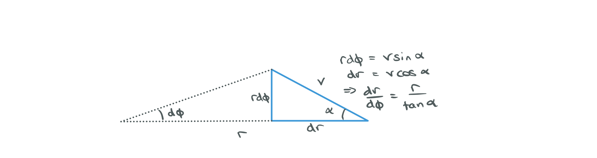
ii)
def escape(t, y): return y[1] - 1/100
escape.terminal = True

def horizon(t, y): return y[1] - 1
horizon.terminal = True

def geodesic(u, udot, phi_max, r_s = 1, max_step = 0.1):
    """
    Integrates f(phi, y = (udot(phi), u(phi))) given inital data u and udot. For phi in (0, phi_max).
    The stepsize is variable but will not be larger than max_step so this can be used to get smoother plots of the trajectory.
    Returns phi, u, o such that (u[i], phi[i]) is the ith point along the trajectory.
    o is the full result object returned by solve_ivp which contains, among other things, information about events that occured on the trajectory.

    The number of points returned depends on the initial conditions, step size and stopping criteria.

    Stops if r grows larger than 100 * r_s, i.e the ray is going to infinity
    or if r < 1 in which case the ray has crossed the event horizon.
    """
    def f(phi, y): return np.array([-y[1]*(1 - 3/2 * r_s * y[1]), y[0]])
    o = solve_ivp(
             fun = f,
             t_span = (0, phi_max),
             y0 = np.array([udot, u]),
             max_step = max_step,
             events = [escape, horizon],
             )
    return o.t, o.y[1], o

fig, axes = plt.subplots(ncols = 2, figsize = (14,7))

r = 5
s = 5


for r_s, ax in zip([0,1],axes):
    ax.set(xlim = (-s,s), ylim = (-s,s))

    for alpha in np.linspace(0.01, pi/2 ,50):
        rdot = -r/np.tan(alpha)

        u, udot = r_rdot_to_u_udot(r, rdot)
        phi, u, o = geodesic(u, udot, phi_max = 10, r_s = r_s)
        x, y = phi_u_to_xy(phi, u)

        color = "blue" if len(o.t_events[0]) > 0 else "red"

        ax.plot(x,y, color = color)

    phi = np.linspace(0,2*np.pi,100)
    ax.plot(1*np.cos(phi), 1*np.sin(phi), linestyle = '-', color = 'black', label = "Schwarzchild Radius")
    ax.legend()

axes[0].set(title = "Flat Spacetime")
axes[1].set(title = "Schwarzchild Spacetime");

At this point we should stop and think about what this is. We're calculating geodesics emanating from an observer at some point outside the horizon. If we want to interpret what this means about how a black hole looks we have to be careful:
1) When doing raytracing we're assuming the geodesics are reversible, that is: light could follow a path from the surface of the horizon to the observer. You'll have to take my word that this is true in this case, though you can easily see that it isn't true for points inside the event horizon. 2) The other thing to note is that when matter falls into a black hole, light that it emits will appear more and more redshifted until it's essentially invisible. We're not going to account for that here.
That being said, the above plots tell us two things about what black hole look like:
1) The horizon appears larger than it actually is. 2) We are able to see light that is emitted from the back, side and actually all the way around the hole. If you add more rays you'll see there's no limit to how many loops the light rays can make, it just requires more and more tuning of the angle. This means that at the edge of our image of the hole we're going to see a lot of copies of the hole all smushed together.
Question 6
Now we're going to move out of this 2D plane into 3D, let's define $\alpha$ as before and also introduce $\beta$ which will measure rotation about the line between the observer and the origin and $\gamma$ which will be the value of $\phi$ when the ray intersected the event horizon.
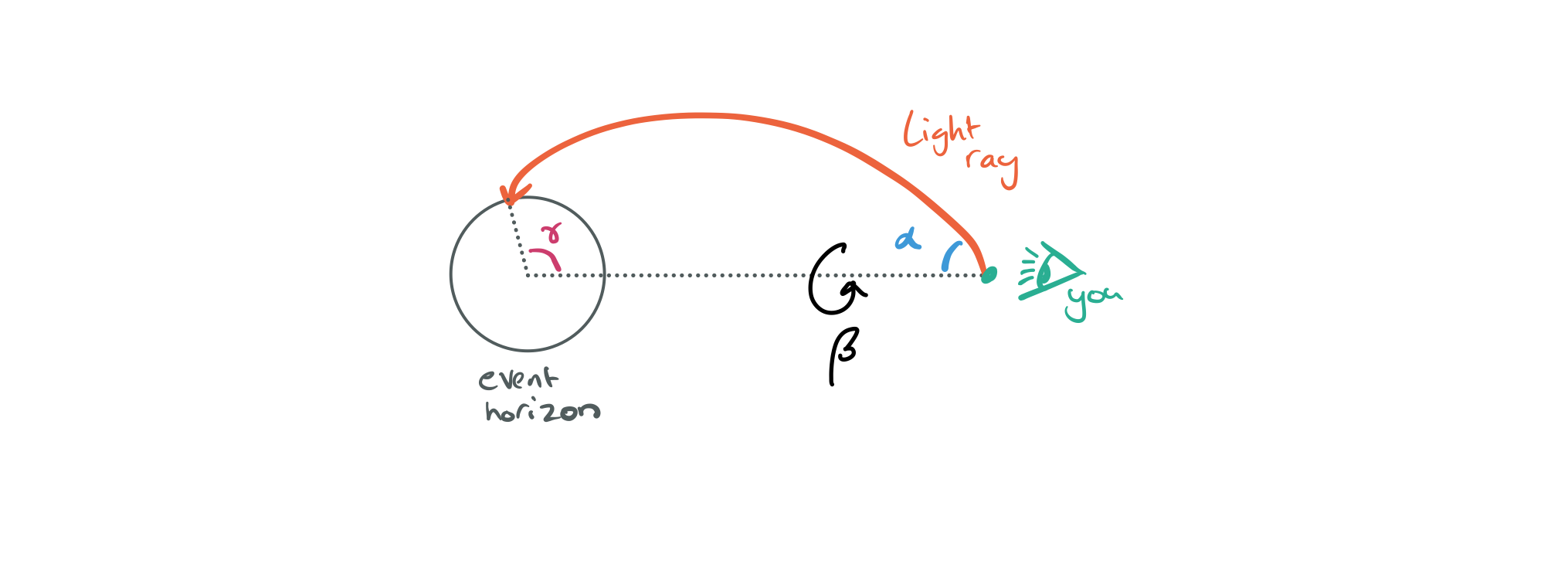
We'll cheat a bit, because of the high symmetry of the (non-rotating) black hole and the fact we're looking at it axially, all we really need to know is $\gamma(\alpha)$, $\beta$ just rotates everything. The rest is just coordinate transorms, incredible tedious ones at that.
Use your geodesic code to make a lookup table for $\gamma(\alpha)$ with $\alpha$ between 0.01 and $\pi$ for both Schwarzchild $r_s = 1$ and flat $r_s = 0$ spacetime. In principle we could also collect information about the escaped rays but I'll leave that as an exercise for the reader.
Answer 6
r_obs = 3

def compute_interpolation(interp_alphas, r_obs, r_s):
    interp_gamma = np.full(shape = len(interp_alphas), fill_value = np.NaN)

    for i, alpha in enumerate(interp_alphas):
        rdot = -r_obs/np.tan(alpha)
        u, udot = r_rdot_to_u_udot(r_obs, rdot)
        phi, u, o = geodesic(u, udot, phi_max = 10, max_step = np.inf, r_s = r_s)

        #if the ray doesn't hit the horizon, stop.
        if len(o.t_events[1]) == 0: break

        #otherwisee save the gamma where it hit the horizon.
        interp_gamma[i] = o.t_events[1][0]

    #we stopped computing at i, so cut everthing else off
    return interp_alphas[:i], interp_gamma[:i]

fig, axes = plt.subplots(ncols = 2, figsize = (16,8))

for i, r_obs in enumerate([70, 1.5]):
    interp_alphas = np.linspace(0.001,pi/2, 1000) # the range of alpha that we will use
    schwarzchild_alphas, schwarzchild_gammas = compute_interpolation(interp_alphas, r_obs, r_s = 1)
    flat_alphas, flat_gammas = compute_interpolation(interp_alphas, r_obs, r_s = 0)
    ax = axes[i]


    ax.plot(schwarzchild_alphas, schwarzchild_gammas, label = "Schwarzhild")
    ax.plot(flat_alphas, flat_gammas, label = "Flat Spacetime")

    ax.axvline(x = flat_alphas[-1], linestyle = '--', label = "Max alpha in flat space")
    ax.axhline(y = flat_gammas[-1], linestyle = '-.', label = "Max gamma in flat space")
    ax.legend()
    ax.set(ylabel = "gamma", xlabel = "alpha")

axes[1].set(xlim = (0, 1), ylim = (0, 7), title = "Very close to the horizon, r_obs = 3")
axes[0].set(xlim = (0, 0.07), ylim = (0, 7), title = "Far from the horizon, r_obs = 30");

From the above we see that the functions are similar when the rays are travelling almost directly towards the centre of the hole but the black hole is visible for a much larger range of $\alpha$ than it would be in flat spacetime (If it were just a sphere rather than a gravitationally massive body).
Question 7
Now we'll put together the funtion we computed in qustion 6 to render an image of the surface of a black hole as viewed at some distance. To give us some reference we're going to texture the surface of the event horizon with an image of the earth surface, this is terrible unphysical since the earth is not a black hole, it's not emissive, etc etc but it's more interesting that just plotting lines of constant $\phi$ and $\theta$.
We'll take the image below as our convention for how to put coordinates on a sphere though I'll be using radians instead of degrees in the code.
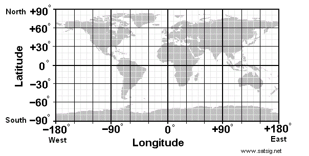
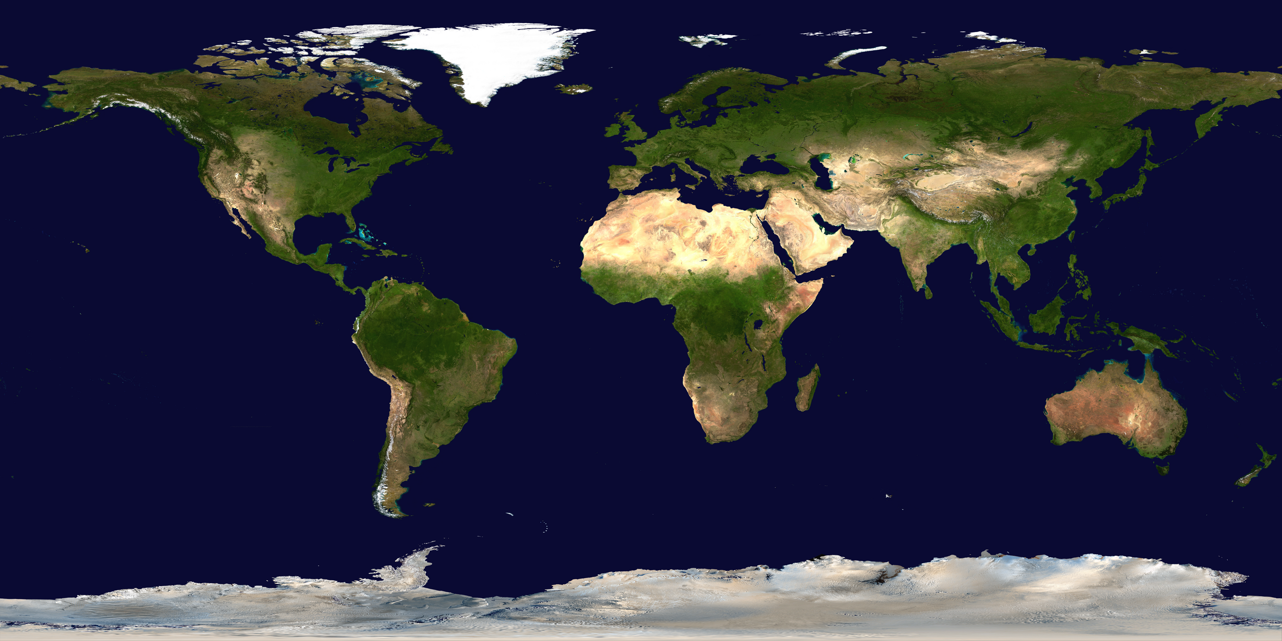
This code is not that interesting to write so I'll just give it to you, we load in an image (which you need to download from here) and then use an interpolater to get a function that maps lat,lon points to colors earth([(lat0,lon0), (lat1,lon1)...]) -> [(r0, g0, b0), (r1, g1, b1)...]
from matplotlib import image
import scipy.interpolate
#get this from https://upload.wikimedia.org/wikipedia/commons/thumb/2/23/Blue_Marble_2002.png/2560px-Blue_Marble_2002.png
im = image.imread("./Blue_Marble_2002.png")
print(im.shape)


lat = np.linspace(-pi/2, pi/2, im.shape[0])
lon = np.linspace(-pi, pi, im.shape[1])

latv, lonv = np.meshgrid(lat, lon, sparse=False, indexing='ij')

earth_interp = scipy.interpolate.RegularGridInterpolator([lat, lon], im, bounds_error=False)

def to_points(xv, yv): return np.array([xv, yv]).transpose((1,2,0))
def wrap_lon(phase): return (phase + pi) % (2 * pi) - pi #wraps to the interval -pi, pi
def wrap_lat(phase): return (phase + pi/2) % (pi) - pi / 2 #wraps to the interval -pi/2, pi/2

def earth(lat, lon):
    points = to_points(wrap_lat(lat), wrap_lon(lon))
    return np.clip(earth_interp(points), 0.0, 1.0)

fig, axes = plt.subplots(figsize = (20,20))
plt.imshow(earth(latv, lonv))
(1280, 2560, 3)

<matplotlib.image.AxesImage at 0x7f94be82ad10>

I'm going to walk you through this a little bit because the process of rendering this image is a little fidly and look me a while to get right.
First we want to define the bounds of our image, for want of better names I'll call the coordinates x and y but really they measure the angles of rays hitting our observers eye. We'll choose $2\pi/3$ as the persons maximum field of view.
fov = 2*pi/3 #field of vieew

#define coordinates for our image window
x = np.linspace(-fov/2, fov/2, 500)
y = np.linspace(-fov/2, fov/2, 500)
Next we define a 'mesh' this means that while x and y are just arrays [x0, x1 ...] , xv and yv have two dimensions such that (xv[i,j], yv[i,j]) is the coordinate of the (i,j) grid point. This allows us to do fast numpy things like r = np.sqrt(xv**2 + yv**2) which gives us a variable defined over the image plane equal to the distance from the origin.
xv, yv = np.meshgrid(x, y, sparse=False, indexing='ij')
Next we define r and $\phi$ in the image plane. If you look at the diagram from question 6 you should be able to convinve yourself that it makes sense to define $\alpha = r$ and $\beta = \phi$
r = np.sqrt(xv**2 + yv**2) #ranges from 0 to pi/3
phi = np.arctan2(xv, yv) #ranges from -pi to pi
#we map alpha as define above onto r and beta onto phi
alpha = r
beta = phi
Now we actually map alpha onto gamma, here spacetime is a function you need to write that maps alpha onto gamma according to the spacetime you're in. You want to interpolate the data you got from question 6. The pi/2 - spacetime(alpha)is because we're measuring our azimuthal angles from the equator rather than from the poles.
def spacetime(x): return x #a dummy function that you need to fill in
gamma = pi/2 - spacetime(alpha)
beta = beta
And finally, just so that we can view the earth from the side rather than only at one of the poles, we'll map to 3D cartesian coordinates, rotate the axes and then map back. Now$(\phi, \theta)$ are the longitude and lattitude on the earth so we can map straight to an image pixel and we're done!
def polar_to_cart(r, phi, theta):
    """
    Convert a spherical polar coordinate system
    (r, phi theta) 0 < r, -pi < phi < pi, -pi/2 < theta < pi/2
    into Cartesian x,y,z coordinates

    NB:
    Phi measures rotations about the z axis
    Theta is the angle above or below the xy plane
    This is slightly different from the typical definition where theta is the angle with the z axis.
    """
    return r * np.cos(phi) * np.cos(theta), r * np.sin(phi)*np.cos(theta), r * np.sin(theta)

def cart_to_polar(x,y,z):
    """
    Reverse the above transformation.
    Uses the convention that phi ranges from -pi to pi
    and theta ranges from -pi/2 to pi
    """
    r = np.sqrt(x**2 + y**2 + z**2)
    theta = np.arcsin(z / r)
    phi = np.arctan2(y,x)
    return r, phi, theta

x,y,z = polar_to_cart(r = 1, phi = beta, theta = gamma)
_, phi, theta = cart_to_polar(x,-z,y)
Can you put all that together to make an image of the surface of the earth if the surface of the earth also happend to be the event horizon of a black hole? (Terms and conditions apply, this can't actually happen, gravitational redshift is ignored etc etc)
I wouldn't blame you for skipping to the solution on this one, it's a bit tricky but the payoff is nice.
Answer 7
r_obs = 3
interp_alphas = np.linspace(0.001,pi/2, 1000) # the range of alpha that we will use
schwarzchild_alphas, schwarzchild_gammas = compute_interpolation(interp_alphas, r_obs, r_s = 1)
flat_alphas, flat_gammas = compute_interpolation(interp_alphas, r_obs, r_s = 0)

#these two functions interpolate the gamma(alpha) functions we calculated earlier
#right = np.NaN tells them to return NaN if alpha is too large and the ray doesn't hit.
def schwarzchild_gamma(alpha):
    shape = alpha.shape
    return np.interp(alpha.flatten(), schwarzchild_alphas, schwarzchild_gammas, right = np.NaN).reshape(shape)

def flat_gamma(alpha):
    shape = alpha.shape
    return np.interp(alpha.flatten(), flat_alphas, flat_gammas, right = np.NaN).reshape(shape)

fig, rows = plt.subplots(nrows = 2, ncols = 3, figsize = (15,10))

for axes, name, spacetime in zip(rows, ["Flat", "Schwarzchild"],[flat_gamma, schwarzchild_gamma]):
    fov = 2*pi/3 #field of vieew

    #define coordinates for our image window
    x = np.linspace(-fov/2, fov/2, 500)
    y = np.linspace(-fov/2, fov/2, 500)

    #make them into grids
    xv, yv = np.meshgrid(x, y, sparse=False, indexing='ij')

    #define r and phi for our image window
    r = np.sqrt(xv**2 + yv**2) #ranges from 0 to pi/3
    phi = np.arctan2(xv, yv) #ranges from -pi to pi

    #we map alpha as define above onto r and beta onto phi
    alpha = r
    beta = phi

    gamma = pi/2 - spacetime(alpha)
    beta = beta


    x,y,z = polar_to_cart(r = 1, phi = beta, theta = gamma)
    _, phi, theta = cart_to_polar(x,-z,y)

    axes[0].imshow(earth(gamma, beta))
    axes[1].imshow(earth(-gamma, beta))
    axes[2].imshow(earth(theta, phi))

    for a in axes:
        a.axis('off')
        a.set(title = name)
/Users/tom/miniconda3/lib/python3.7/site-packages/ipykernel_launcher.py:17: RuntimeWarning: invalid value encountered in remainder
/Users/tom/miniconda3/lib/python3.7/site-packages/ipykernel_launcher.py:16: RuntimeWarning: invalid value encountered in remainder
  app.launch_new_instance()
